Welcome

How to cite this book

If you use this book in your work, please cite it as:

APA: Chaudhri, A. (2026). Real-Time Vehicle Tracking with Neo4j, Databricks Lakebase and OpenStreetMap. Self-published. https://realtime-vehicle-tracking.github.io/

BibTeX:

@online{chaudhri2026vehicletracking,
  author  = {Chaudhri, Akmal},
  title   = {Real-Time Vehicle Tracking with Neo4j, Databricks Lakebase and OpenStreetMap},
  year    = {2026},
  url     = {https://realtime-vehicle-tracking.github.io/},
  urldate = {2026-08-28}
}

Cover

License

Copyright

Copyright © 2026 Akmal Chaudhri. All rights reserved.

Publication Information

First published: August 2026

The latest version of this book, together with updates, errata and additional resources, is available at:

realtime-vehicle-tracking.github.io

Book License

Real-Time Vehicle Tracking with Neo4j, Databricks Lakebase and OpenStreetMap is licensed under the Creative Commons Attribution-NonCommercial-NoDerivatives 4.0 International License (CC BY-NC-ND 4.0).

You are free to copy and redistribute this book in any medium or format under the following conditions:

• Attribution - You must give appropriate credit, provide a link to the license and indicate if changes were made.
• NonCommercial - You may not use the material for commercial purposes.
• NoDerivatives - If you remix, transform or build upon the material, you may not distribute the modified material.

The full license text is available at:

creativecommons.org/licenses/by-nc-nd/4.0

Code License

Unless otherwise stated, all code samples, notebooks, scripts and source files accompanying this book are licensed under the Apache License 2.0.

You are free to use, modify and redistribute this code, including for commercial purposes, subject to the terms of the Apache License 2.0.

The full license text is available at:

apache.org/licenses/LICENSE-2.0

This distinction means that the book’s written content is protected under the Creative Commons license, while the accompanying code remains freely available for use, modification and integration into your own projects.

The pre-clipped OpenStreetMap data files are available under the Open Database License (ODbL). See LICENSE-DATA.

Trademarks

Product names, company names and logos mentioned in this book may be trademarks or registered trademarks of their respective owners.

Their inclusion is for identification and educational purposes only and does not imply any affiliation with, sponsorship by or endorsement from the respective trademark holders. All trademarks remain the property of their respective owners.

Disclaimer

The information in this book, including all code samples, scripts and notebooks, is provided “as is” without warranty of any kind, express or implied.

The author makes no representations or warranties regarding the accuracy, completeness, reliability or suitability of the information contained herein for any particular purpose.

Examples are provided solely to illustrate technical concepts, patterns and software architectures.

Readers are responsible for independently validating all code, configurations and recommendations before using them in production environments.

To the fullest extent permitted by law, the author shall not be liable for any direct, indirect, incidental, special, consequential or other damages arising from the use of or inability to use, the information, code or techniques described in this book.

Attribution

Map data © OpenStreetMap contributors, available under the Open Database License.

Regional OSM data files sourced from Geofabrik.

About the Author

Akmal Chaudhri is a technical leader, educator and author with extensive experience in databases, AI and developer relations. He specializes in technical writing, developer education and community building, helping engineers and organizations understand and adopt complex technologies through clear, practical and engaging content. He is a frequent international speaker, a published author and a contributor to industry discussions on data platforms, AI and software development.

Today, Akmal works in developer education at Neo4j, where he focuses on technical content, workshops and community initiatives. While his professional role has evolved, this book represents an independent exploration of various data platforms.

Based in the United Kingdom, Akmal continues to work at the intersection of databases, AI and developer tooling, helping developers build modern data-driven applications.

For book updates, code samples and additional resources, visit the Book website.

To connect professionally or follow his latest work, visit LinkedIn.

Real-time vehicle tracking with Neo4j, Databricks Lakebase and OpenStreetMap

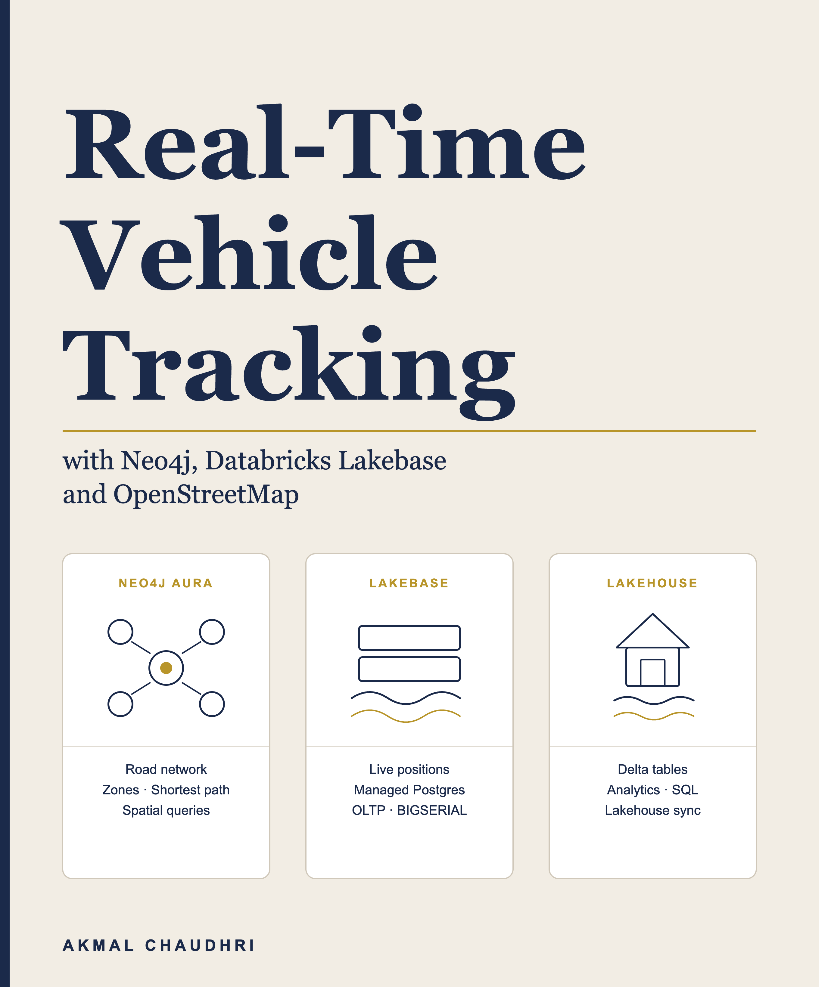
This book builds a real-time fleet operations dashboard using three database systems:

1. Neo4j Aura for the road network graph.
2. Databricks Lakebase for live vehicle positions.
3. Databricks Lakehouse for historical analytics.

Ten simulated vehicles move around a city following real road connections loaded from OpenStreetMap. Two Streamlit dashboards show live positions and analytics.

The primary demo uses the London Borough of Merton. Additional example configurations are provided for San Francisco and Singapore. The whole system is driven by a single YAML configuration file.

How the code is organized

All runnable code lives in the code/ directory alongside config.yaml. The same directory holds the two example configs for San Francisco and Singapore, config_validator.py and the two Streamlit apps, app.py and analytics_app.py. The simulator script is written by the Chapter 5 notebook.

The chapter markdown files live in src/.

Notebooks are numbered to match the chapters – 02_road_network.ipynb corresponds to Chapter 2, and so on. The one notebook for Chapter 1, 01_prepare_osm.ipynb, is optional. It prepares the local OpenStreetMap files for San Francisco, Singapore or a new city, and Merton doesn’t need it.

Chapter 1: Architecture and Setup

What we’re building

Real-time vehicle tracking sits at the intersection of three distinct data problems:

1. Graph problem – what’s the shortest route between two points on an actual road network and which zones are reachable from where?
2. Operational problem – where are my vehicles right now and where have they been?
3. Analytical problem – which areas of the city are seeing the most activity and which roads carry the most traffic?

Each of those problems has a natural home in a different kind of database. That’s the core idea behind this book. We’re not going to use one database and make it do everything. We’re going to use three and let each one do what it does best.

The system we’ll build is a fleet operations dashboard for the London Borough of Merton – a compact urban borough in South London with a dense road network that’s large enough to be interesting but small enough to run on free-tier accounts. Ten simulated vehicles move around the borough following real road connections loaded from OpenStreetMap. A live Streamlit dashboard shows their positions, trails, the nearest driver to any zone and the shortest path between any two zones. A separate analytics dashboard shows zone activity over time and which named roads carry the most traffic.

We’ll also show how to adapt the entire system to a different city by changing a single configuration file. Additional example configuration files are provided for San Francisco and Singapore.

The three-system architecture

The architecture has three layers, each serving a different purpose.

Neo4j Aura is the graph layer. It holds the road network for Merton – 3,212 intersections and 7,296 road segments loaded from OpenStreetMap via the OSMnx library. Aura answers the questions that a relational database handles with difficulty:

• What’s the shortest path between two points along drivable roads?
• Which zones border which other zones?
• Which intersections are the most connected hubs of the network?

Each intersection carries a native spatial point, and nearest-neighbor lookups are fast enough to run on every map refresh for a network of this size.

Databricks Lakebase is the operational layer. It’s a fully managed Postgres database, hosted inside Databricks, that accepts the high-frequency position writes from our vehicle simulator. Every two seconds, ten vehicles each write their current coordinates to a vehicle_positions table. Lakebase handles this with standard psycopg2 connectivity, foreign key constraints and BIGSERIAL auto-increment IDs. The token-based authentication enforces a natural session boundary, as each token lasts an hour, which is the right behavior for a demo.

Databricks Lakehouse is the analytics layer. Position data flows from Lakebase into a Delta table, where we run aggregations, such as zone demand over time, position volume trends and the cross-system join that answers “which named roads carry the most traffic?” by combining Lakebase position data with Aura road names.

The relationship between these systems is as follows:

• Aura is where the structure lives – the road graph that neither Lakebase nor Lakehouse knows anything about.
• Lakebase is where data are written, in real time, by the simulator.
• Lakehouse is where we analyze the history that Lakebase accumulates.

Each system has a clear role and none of the roles overlap.

What Aura adds

A natural question is: what does Aura add? We already have a Postgres database. Can’t we just store road network data there too? We could store it there. But querying it could be difficult. The shortest path between two points requires traversing a graph – following edges from node to node, keeping track of visited nodes and finding the sequence with the fewest hops. In SQL this means recursive CTEs, which are slow for deep traversals. In Cypher, Aura’s query language, it’s a single function call. For example:

MATCH (a:Intersection {node_id: $start_id}), (b:Intersection {node_id: $end_id})
MATCH path = shortestPath((a)-[:ROAD*..300]->(b))
RETURN length(path) AS hops

The zone adjacency queries are similarly clean. “Which zones can be reached within two hops from Morden?” is a short Cypher query. In SQL it would require multiple self-joins or a recursive CTE that grows in complexity with each additional hop.

Also, the road network is a graph. Intersections are nodes. Roads are edges. The connectivity between them is the point. Storing that as rows and columns in a relational table is possible but goes against the natural structure of the data.

The configuration file

Every city-specific value in the system lives in a single YAML file called config.yaml. The zone definitions, zone adjacency, vehicle assignments, map coordinates, schema name and OpenStreetMap place name all come from this file. For cities that use a local OSM file, the file name, source URL and bounding box live there too. Switching from London to San Francisco or Singapore means copying a different config file into place and re-running the notebooks.

There are three example configs:

1. config.yaml – the London Borough of Merton (the default)
2. config_sf.yaml – five neighborhoods in central and southeastern San Francisco
3. config_sg.yaml – five planning areas in central Singapore

The supporting code in config_validator.py validates the config file on load and raises clear errors if anything is missing or malformed.

One optional notebook accompanies this chapter. 01_prepare_osm.ipynb downloads and clips an OpenStreetMap file for cities that use a local file instead of the Overpass API. The clipped files for San Francisco and Singapore are already in the repository, so you only need this notebook to regenerate them or to prepare your own city. Merton doesn’t need it. If you do run it, run it before 02_road_network.ipynb.

What you’ll need

To follow along you’ll need accounts and access to these services:

1. Neo4j Aura – the free tier is sufficient. Create an account at Get Started for Free and note your URI, username and password. Use an instance you’re happy to wipe, because the notebooks clear the database before loading.
2. Databricks – a Free Edition account gives us access to both Lakebase and Lakehouse. Create an account at Databricks Free Edition. Create a Lakebase project named vehicle-tracker and a SQL warehouse before running the notebooks.
3. Python – the code was tested using Python 3.12 and it may not work on more recent versions of Python. The notebooks run in a local Jupyter environment. A virtual environment is highly recommended. For example:

python3 -m venv ~/vehicle-tracker-env
source ~/vehicle-tracker-env/bin/activate

All dependencies are installed using %pip install cells at the top of each notebook, with pinned versions for stability.

Environment variables

Credentials are passed to notebooks and the Streamlit applications using environment variables. Set these before starting Jupyter:

# Neo4j Aura
export NEO4J_URI="neo4j+s://xxxx.databases.neo4j.io"
export NEO4J_USERNAME="your-username"
export NEO4J_PASSWORD="your-password"

# Databricks Lakebase
export LAKEBASE_HOST="ep-xxxx.database.eu-west-1.cloud.databricks.com"
export LAKEBASE_USER="your-databricks-email"
export LAKEBASE_TOKEN="your-oauth-token"
export LAKEBASE_DBNAME="databricks_postgres"

# Databricks Lakehouse
export DATABRICKS_SERVER_HOSTNAME="dbc-xxxx.cloud.databricks.com"
export DATABRICKS_HTTP_PATH="/sql/1.0/warehouses/xxxx"
export DATABRICKS_TOKEN="your-personal-access-token"

Note that LAKEBASE_TOKEN expires after one hour. This is by design – it’s Databricks’s authentication model for OAuth-based access and it gives us a natural session boundary. When it expires, we need to generate a fresh token from the Lakebase Connect dialog in the Databricks UI and update the LAKEBASE_TOKEN environment variable.

Chapter overview

Here’s what each chapter covers:

Chapter 2: The Road Network walks through loading the Merton road network from OpenStreetMap into Aura using OSMnx. We’ll cover the data cleaning required to handle the quirks of OSM data, such as list-valued properties, duplicate edges and missing speed limits. We’ll also describe the Aura schema that makes spatial queries efficient.

Chapter 3: Zones and Graph Queries defines the five zones that divide the borough, assigns each intersection to its zone and builds the zone adjacency graph. We’ll show the Cypher queries that make the zone topology useful, such as nearest neighbors, multi-hop reachability and complex intersection counts.

Chapter 4: The Operational Layer sets up the Lakebase tables that hold live vehicle data. We’ll cover the table design, the indexes that make time-series queries fast and the credentials for connecting from Python.

Chapter 5: The Simulator writes a vehicle simulator that loads the road network from Aura, places ten vehicles in their home zones and moves each one along Breadth-First Search (BFS)-computed shortest paths. The simulator runs as a background process and writes position updates to Lakebase every two seconds.

Chapter 6: The Streamlit Apps builds two Streamlit dashboards. The first one shows vehicles moving on a live map with trail history and shortest path queries. The second one connects to Lakehouse to show zone activity trends and road segment traffic, updated every 30 seconds.

Chapter 7: Bringing It All Together covers the full system running end-to-end and ideas for going further.

Let’s start by loading the road network.

Chapter 2: The Road Network

What we need from the road network

The road network is the foundation of the entire system. Without it, we can’t route vehicles, compute shortest paths between zones or tell a vehicle where to go next. Everything the simulator and the Streamlit application do depends on having an accurate, connected graph of the roads in a city.

We specifically need:

• Every road intersection as a node, with its GPS coordinates.
• Every drivable road segment as a directed edge, with its name, road type, speed limit and length.
• A spatial index on intersection coordinates to support location lookups, such as finding the nearest intersection to a GPS position.
• A connected graph, with no isolated subgraphs, so every vehicle can reach every other zone via some sequence of road segments.

OpenStreetMap gives us the raw data. OSMnx gives us the tools to download it, clean it and convert it to a graph we can load into Aura.

The Aura graph model

The road network maps naturally to Aura’s property graph model. Here’s what we’re storing:

(:Intersection {node_id, lat, lon, street_count, location})
    -[:ROAD {osmid, u, v, name, highway, maxspeed, oneway, length_m}]->
(:Intersection)

Each Intersection node represents a road junction, which is a point where two or more roads meet. The location property stores an Aura point() object, which enables native spatial queries (nearest-neighbor lookup, distance calculation) without any additional libraries.

Each ROAD relationship represents a directed road segment between two intersections. A one-way street from A to B is stored as a single relationship A -> B. A two-way street is stored as two relationships: A -> B and B -> A. The highway property holds the OSM road classification (primary, residential, motorway and so on) and maxspeed holds the posted speed limit where OSM data are available. The osmid property is stored as a string.

Downloading the road network

For Merton, we use OSMnx’s graph_from_place() function, which geocodes the place name via Nominatim, finds the boundary polygon in OpenStreetMap and downloads all drivable road segments within it:

G = ox.graph_from_place("London Borough of Merton, UK", network_type="drive")

The network_type="drive" filter keeps only roads that cars can use, excluding footpaths, cycleways and pedestrian areas. By default OSMnx also drops road segments that aren’t part of the largest connected component, which helps keep the graph connected.

For alternate cities, such as San Francisco and Singapore, where neighborhood polygon boundaries are either unavailable or produce disconnected subgraphs, we use a different approach: download a regional OSM data file from Geofabrik and clip it to a bounding box using pyrosm. This is covered in notebook 01_prepare_osm.ipynb, which you only need to run if you want to regenerate the clipped file or prepare your own city.

The city config file (config.yaml) tells 02_road_network.ipynb which approach to use:

city:
  osmnx_place: "London Borough of Merton, UK"  # Merton -- direct download
  # osm_file: "singapore-central.osm.pbf"      # Singapore -- local file

If osm_file is present, the notebook loads from the local clipped file. Otherwise it uses graph_from_place(). The notebook also accepts osmnx_place as a list of place names and composes the individual graphs with nx.compose(), but none of the example configs use this.

Cleaning the data

OSMnx returns a MultiDiGraph, which is a directed graph where edges can have multiple attributes, some of which are lists rather than scalars. In the OSM data model, a single road segment can carry multiple OSM tag values when the underlying data are ambiguous or inconsistent.

Before loading into Aura, we need to clean three things:

1. List-valued properties. The osmid, name, highway and maxspeed fields can be Python lists rather than single values. We take the first element in each case:

def flatten(val):
    if isinstance(val, list):
        return val[0]
    return val

2. Speed limit strings. OSM stores maxspeed as a string ("50 mph" or just "50") rather than a number. We parse it to a number, stripping the unit suffix. Missing values become None, so the column is stored as floating point, which is why speed limits show as 20.0 rather than 20:

def parse_maxspeed(val):
    if val is None or (isinstance(val, float) and pd.isna(val)):
        return None
    val = flatten(val)
    try:
        return int(str(val).replace(" mph", "").strip())
    except (ValueError, AttributeError):
        return None

3. NaN values. Pandas uses float('nan') for missing values, but the Neo4j Python driver doesn’t accept NaN. We convert all NaN values to None before loading:

rows = df.where(pd.notnull(df), None).to_dict("records")

Deduplicating edges

OSMnx assigns the same osmid to multiple edges in two cases:

1. Bidirectional roads, where the same OSM way appears as both A -> B and B -> A. These differ in u and v, so we keep both as separate directed relationships.
2. Segmented ways, where a single named road is split into multiple segments sharing one OSM ID.

Only the second case needs deduplicating. The composite key osmid + u + v (where u and v are the source and target node IDs) is usually unique, but not always, as some split ways produce multiple segments with the same u, v and osmid but different lengths. We deduplicate by keeping the longest segment for each (osmid, u, v) triple:

edges_clean = (
    edges_clean
    .sort_values("length_m", ascending=False)
    .drop_duplicates(subset=["osmid", "u", "v"], keep="first")
)

This reduces Merton’s 7,335 raw edges to 7,296 clean edges with duplicates removed.

Loading into Aura

We load nodes and edges in separate passes, using MERGE to make the operation idempotent. Running the notebook twice won’t create duplicate nodes.

Nodes. Each intersection becomes an Aura node, with a uniqueness constraint on node_id created beforehand:

CREATE CONSTRAINT intersection_node_id IF NOT EXISTS
FOR (i:Intersection) REQUIRE i.node_id IS UNIQUE

The node load itself looks like this:

UNWIND $rows AS row
MERGE (i:Intersection {node_id: row.node_id})
SET i.lat          = row.lat,
    i.lon          = row.lon,
    i.street_count = row.street_count,
    i.location     = point({latitude: row.lat, longitude: row.lon})

The location property stores a native Aura spatial point, which enables the point.distance() function used later for nearest-driver queries.

Edges. Each road segment becomes a ROAD relationship. The composite MERGE key uses osmid, u and v together to uniquely identify each directed edge:

UNWIND $rows AS row
MATCH (a:Intersection {node_id: row.u})
MATCH (b:Intersection {node_id: row.v})
MERGE (a)-[r:ROAD {osmid: row.osmid, u: row.u, v: row.v}]->(b)
SET r.name     = row.name,
    r.highway  = row.highway,
    r.maxspeed = row.maxspeed,
    r.oneway   = row.oneway,
    r.length_m = row.length_m

We load in batches of 500 rows at a time, using a progress bar to track progress. For Merton this load is quite fast. For San Francisco and Singapore it takes longer.

Clearing before reload

Warning: The reset deletes everything in the database, including data, constraints and indexes that don’t belong to this book. Run it only against an instance you’re happy to wipe, such as a fresh Aura Free instance created for this project.

When switching cities, we need to reset the database before loading a new one. The reset drops all constraints, drops all non-lookup indexes and then deletes every node and relationship in batches of 1,000. We skip the lookup indexes because Neo4j manages those itself. The reset runs before the constraint and index setup, so the notebook always starts from a clean slate:

def clear_database(session):
    # Drop all constraints
    constraints = session.run("SHOW CONSTRAINTS YIELD name RETURN name").data()
    for c in constraints:
        session.run(f"DROP CONSTRAINT {c['name']} IF EXISTS")

    # Drop all non-lookup indexes
    indexes = session.run("""
        SHOW INDEXES YIELD name, type
        WHERE type <> 'LOOKUP'
        RETURN name
    """).data()
    for idx in indexes:
        session.run(f"DROP INDEX {idx['name']} IF EXISTS")

    # Delete all nodes and relationships in batches
    while True:
        result = session.run("""
            MATCH (n) WITH n LIMIT 1000
            DETACH DELETE n
            RETURN count(*) AS deleted
        """)
        if result.single()["deleted"] == 0:
            break

    print("Database cleared.")

with driver.session() as session:
    clear_database(session)

The spatial index

The POINT INDEX on location is created before loading nodes:

CREATE POINT INDEX intersection_location IF NOT EXISTS
FOR (i:Intersection) ON (i.location)

Creating it before the data load means the index is populated incrementally as nodes are inserted.

Verifying the result

After loading, we verify the counts match expectations and inspect the longest named roads:

Intersections : 3,212
Roads         : 7,296

Longest named roads:
  Home Park Road                 residential  20.0       1013.41 m
  Home Park Road                 residential  20.0       1013.41 m
  Croydon Road                   primary      30.0       960.11 m
  Croydon Road                   primary      30.0       960.11 m
  Lynmouth Avenue                residential  20.0       828.92 m

The duplicate entries reflect different directed edges sharing the same display attributes. For example, two segments of a road traveling in opposite directions. The graph data in Aura is correct.

For Merton, we expect 3,212 intersections and 7,296 roads after deduplication. Home Park Road, at over a kilometer, is a residential street. Croydon Road is a primary road with a 30 mph limit. OpenStreetMap is edited continuously, so your counts may differ slightly from the ones shown here.

Alternate cities

For San Francisco and Singapore, the road network is loaded from a pre-clipped OSM file rather than using the Overpass API. The 01_prepare_osm.ipynb notebook handles downloading the regional file from Geofabrik and clipping it to the bounding box defined in the city config. You can regenerate these files at any time by running that notebook with the appropriate config.

The clipped files are included in the GitHub repo, so you won’t need to run the prepare notebook.

San Francisco’s graph is larger than Merton’s because the area covered is larger and its road network is denser. Singapore’s graph is of a broadly similar size. Both are clipped to a single bounding box, which should give one connected graph. The verification step in 01_prepare_osm.ipynb reports the number of strongly connected components, so you can confirm this for yourself.

Gotchas

OSMnx version compatibility. OSMnx and Shapely versions need to be compatible with each other. Older Shapely releases were built against an earlier major version of NumPy and can fail with a TypeError when OSMnx calls union_all() internally. Pin Shapely to the version in the notebook’s install cell, which is known to work.

List-valued edge properties. OSMnx can return osmid, name, highway and maxspeed as Python lists rather than scalars for some edges. Always flatten before loading. The flatten() helper takes the first element of any list and returns non-list values unchanged.

NaN vs None. The Neo4j Python driver doesn’t accept float('nan'). Call df.where(pd.notnull(df), None) before converting to records.

Edge deduplication. The composite key osmid + u + v is not always unique. Sort by length descending and drop duplicates before loading.

Speed limits in alternate cities. OSM stores speed limits as numbers, sometimes with a unit suffix, and the unit depends on the country. The UK and the US use mph, whereas most other countries, including Singapore, use km/h. The field name is the same, so the notebook stores the number as given and doesn’t convert it.

pbf format. Geofabrik distributes OSM data in Protocol Buffer format (.osm.pbf). This is a binary format that OSMnx’s graph_from_xml() function can’t read directly, as it expects plain OSM XML. Use pyrosm to read .pbf files.

nx.compose() produces disconnected subgraphs. Composing multiple neighborhood polygon graphs with nx.compose() can produce isolated subgraphs if the constituent polygons don’t share road edges at their boundaries. This causes shortestPath() to return no result between nodes in different subgraphs. Use pyrosm with a bounding box to get a single connected graph instead.

Not all place names have OSM polygon boundaries. ox.graph_from_place() requires Nominatim to return a polygon boundary for the place name. Neighborhood names in particular often return only a point. Test with ox.geocode_to_gdf(place) and check that geom_type is Polygon or MultiPolygon before using a place name in your config.

nx.compose() node count is misleading. len(G.nodes) on the first graph in a compose chain returns only that graph’s node count. After composing multiple graphs, Aura receives the full union of all node IDs. The final Aura intersection count is correct; the intermediate len(G.nodes) is not.

Chapter 3: Zones and Graph Queries

Why zones?

The road network we loaded in Chapter 2 is a graph of thousands of intersections connected by thousands of directed road segments. That’s a detailed and accurate model of Merton’s road network, but it’s not enough for a vehicle tracking system on its own.

A dispatcher needs to think in terms of areas, not individual intersections. “Send the nearest vehicle in Colliers Wood to the pickup in Mitcham” is a meaningful instruction. “Send the vehicle at node 65304090 to node 229523558” is not. We need to group the road network into named zones that the simulator and the dashboard can both reason about.

We also need to know which zones border which other zones. The simulator uses this to decide where to send a vehicle next, with a 70% chance of choosing a destination in the vehicle’s home zone or an adjacent zone and a 30% chance of choosing one anywhere in the borough. Without an explicit zone adjacency graph, the simulator would have to compute this at runtime from intersection coordinates, which is slower and more error-prone.

The zone model

We define five logical zones for Merton, each as a simple bounding box:

These are logical simplified zones for the demo, not official neighborhood boundary polygons. Merton’s Local Plan recognizes a richer set of neighborhoods including South Wimbledon, Wimbledon Park, Merton Park and Lower Morden, none of which are represented here. The bounding boxes are a deliberate simplification that keeps the configuration transparent and easy to adjust.

Intersections that fall outside all five boxes are assigned to an Unknown zone automatically. In practice this is just one intersection for Merton.

All zone definitions live in config.yaml. Switching to a different city means changing the config file; the notebook code itself is city-agnostic.

Each zone also has a center point in the config. The centers are reference points on the road network. The apps use them to find the nearest intersection and to measure distances to a zone, and they don’t have to sit inside the bounding box. For Merton, the Raynes Park, Colliers Wood and Morden centers fall outside their own boxes, because the boxes are simplified and the centers sit close to the real locations of those neighborhoods.

Adding zones to Aura

We extend the graph model from Chapter 2 with two new elements:

(:Zone {name, lat_min, lat_max, lon_min, lon_max})
(:Intersection)-[:IN_ZONE]->(:Zone)
(:Zone)-[:ADJACENT_TO]->(:Zone)

Each Zone node stores its bounding box coordinates. The IN_ZONE relationship connects each intersection to its zone. The ADJACENT_TO relationship connects neighboring zones and is stored bidirectionally. We define the pairs by hand in the config so that they form a single connected chain, which means every zone can be reached from every other zone. The chain doesn’t list every pair of boxes that touch.

Assigning intersections to zones

The zone assignment query runs entirely in Cypher. For each intersection, it finds the zone whose bounding box contains the intersection’s coordinates and creates an IN_ZONE relationship:

MATCH (i:Intersection)
MATCH (z:Zone)
WHERE i.lat >= z.lat_min AND i.lat < z.lat_max
  AND i.lon >= z.lon_min AND i.lon < z.lon_max
MERGE (i)-[:IN_ZONE]->(z)
RETURN count(*) AS assigned

Any intersection not matched by this query goes to the Unknown zone. We create that zone first and then assign the leftover intersections to it:

MERGE (z:Zone {name: "Unknown"})

MATCH (i:Intersection)
WHERE NOT (i)-[:IN_ZONE]->()
MATCH (z:Zone {name: "Unknown"})
MERGE (i)-[:IN_ZONE]->(z)

For Merton, this assigns nearly all intersections to named zones and 1 to Unknown.

Zone adjacency

The adjacency relationships define which zones neighbor which others. For Merton, the five zones form a single chain, running Raynes Park -> Wimbledon -> Colliers Wood -> Mitcham -> Morden:

Raynes Park -- Wimbledon -- Colliers Wood -- Mitcham -- Morden

We store adjacency bidirectionally and a single pair [Wimbledon, Colliers Wood] in the config generates two ADJACENT_TO relationships in Aura:

UNWIND $pairs AS pair
MATCH (a:Zone {name: pair.a})
MATCH (b:Zone {name: pair.b})
MERGE (a)-[:ADJACENT_TO]->(b)
MERGE (b)-[:ADJACENT_TO]->(a)

Verifying the zone graph

After loading, we verify both the intersection counts per zone and the adjacency structure:

Intersections per zone:
  Wimbledon       839
  Raynes Park     761
  Mitcham         727
  Colliers Wood   544
  Morden          340
  Unknown         1
  Total           3,212

Zone adjacency:
  Colliers Wood   -> Mitcham, Wimbledon
  Mitcham         -> Colliers Wood, Morden
  Morden          -> Mitcham
  Raynes Park     -> Wimbledon
  Wimbledon       -> Colliers Wood, Raynes Park

Wimbledon has the most intersections. Box size isn’t a reliable guide here, since Morden’s box is nearly as large as Wimbledon’s but holds the fewest. Even so, Morden has more than enough intersections for the simulator to route vehicles meaningfully.

Graph queries on the zone topology

With zones and adjacency loaded, we can ask questions that would be challenging in a relational database.

Which zones border Wimbledon?

MATCH (z:Zone {name: 'Wimbledon'})-[:ADJACENT_TO]->(neighbor:Zone)
RETURN neighbor.name AS zone
ORDER BY zone

Result: Colliers Wood, Raynes Park.

Which zones can a vehicle reach within two hops from Morden?

MATCH (z:Zone {name: 'Morden'})-[:ADJACENT_TO*1..2]->(reachable:Zone)
WHERE reachable.name <> 'Morden'
RETURN DISTINCT reachable.name AS zone
ORDER BY zone

Result: Colliers Wood, Mitcham. Wimbledon and Raynes Park are three and four hops away. The adjacency pairs form one connected chain, so a vehicle starting anywhere can still reach every zone.

How many complex intersections are in Wimbledon?

MATCH (i:Intersection)-[:IN_ZONE]->(z:Zone {name: 'Wimbledon'})
WHERE i.street_count >= 3
RETURN count(i) AS complex_intersections

Result: 635. About 76% of Wimbledon’s 839 intersections connect three or more roads, which reflects the dense residential street grid in this part of London.

Shortest path between zones

The most powerful query the zone graph enables is shortest path between two named zones. The Streamlit application uses this for the “Find shortest path” feature – the user selects two zones, the app finds the nearest intersection to each zone’s center point and then asks Aura for the shortest directed path between them along ROAD relationships:

MATCH (start:Intersection {node_id: $start_id})
MATCH (end:Intersection   {node_id: $end_id})
MATCH path = shortestPath((start)-[:ROAD*..300]->(end))
RETURN [n IN nodes(path) | [n.lon, n.lat]] AS coords,
       length(path) AS hops,
       round(reduce(total = 0.0, r IN relationships(path) |
           total + coalesce(r.length_m, 0.0)) / 1000.0, 2) AS dist_km

The *..300 hop limit prevents the query from running indefinitely on disconnected graphs. For Merton’s well-connected network, shortest paths are typically tens of hops. The result is a sequence of coordinates, in longitude and latitude order, that the Streamlit application draws as a line on the map, together with the hop count and the total length in kilometers.

Finding the nearest intersection to a zone center uses the location point stored on each intersection:

MATCH (i:Intersection)
RETURN i.node_id AS node_id
ORDER BY point.distance(
    i.location,
    point({latitude: $lat, longitude: $lon})
) ASC
LIMIT 1

This runs in milliseconds for a network of this size. As written, the query ranks every intersection by distance, so for a much larger network we’d add a bounding box or distance filter that the POINT INDEX from Chapter 2 can use.

Why store zones in Aura?

We could store zone assignments in Postgres alongside the vehicle positions. The simulator could look up each vehicle’s zone by querying the Lakebase vehicles table. Why put zones in Aura instead?

Two reasons. First, the adjacency queries are natural graph traversals. “Zones reachable within two hops” is a recursive query that SQL handles with CTEs, which can be verbose and slow for deeper traversals. In Cypher it’s a single line with a variable-length path pattern.

Second, the shortest path query crosses zone boundaries. The zone context, which intersections belong to which zone, enriches the result without requiring a join to a separate database. Everything the path query needs is in the same graph.

Zone-awareness in the simulator

The simulator uses zone membership in two ways. At startup, it reads zone membership counts from Aura to confirm the graph loaded correctly:

Zone distribution: {'Wimbledon': 839, 'Raynes Park': 761, ... }

At runtime, it determines the current_zone of each vehicle by checking which zone the vehicle’s current intersection belongs to. This is achieved with an in-memory dictionary built from Aura data at startup, not a live Aura query per tick, so it adds no latency to the simulation loop.

The zone adjacency graph from the config drives the routing bias: 70% of the time a vehicle’s next destination is chosen from its home zone or an adjacent zone and 30% of the time from anywhere in the borough. This creates realistic clustering and vehicles tend to stay in their home area but occasionally make longer cross-borough runs.

Gotchas

Bounding box zones are simplified. The zone bounding boxes are logical demo zones, not official neighborhood boundaries. For Merton, the Local Plan recognizes a richer set of neighborhoods. For Singapore, the URA planning areas have irregular polygon boundaries. For San Francisco, the city publishes official neighborhood boundary maps. The YAML zones are a deliberate simplification for the demo.

Switching cities requires a full Aura wipe. ROAD relationships, Intersection nodes and Zone nodes all need to be cleared before loading a new city. Clearing only ROAD relationships leaves orphaned Intersection nodes from the previous city, which then get mixed into the zone assignment for the new city.

Chapter 4: The Operational Layer

What the operational layer does

Aura holds the road network, which is the structure of the city. But while vehicles are moving, we need somewhere to record what’s actually happening: where each vehicle is right now, where it’s been and what state it’s in. This is the operational layer.

The operational layer needs to handle high-frequency writes. Ten vehicles writing their position every two seconds means up to about 300 writes per minute, sustained for as long as the simulator runs. It also needs to serve the Streamlit application, which reads the latest position of every vehicle on every refresh. These are classic OLTP characteristics: small, frequent reads and writes, low latency and strong consistency.

Databricks Lakebase is a managed Postgres database hosted inside Databricks. It handles the operational workload exactly as a production Postgres instance would, using standard psycopg2 connectivity from Python. Credentials are obtained from the Lakebase Connect dialog in the Databricks UI.

Creating the Lakebase project

Before running this notebook, you’ll need a Lakebase project named vehicle-tracker in your Databricks workspace. The project name is deliberately generic – it’s city-agnostic, so the same project works whether you’re running the Merton, San Francisco or Singapore config. When you switch cities, you re-run this notebook to drop and recreate the tables; the project itself stays the same.

Warning: Running the notebook drops the vehicles, vehicle_positions and trips tables and all the data in them. Only run it against a project you’re happy to reset.

Create the project from the Lakebase section of the Databricks UI.

Setting up credentials

Lakebase connections use an OAuth token as the password. The token expires after one hour. This is intentional – it’s Databricks’s authentication model and it enforces a natural session boundary. For a demo, this is actually useful as it gives us a natural session boundary: after the hour is up, no new connection can be made unless you renew the token. When the token expires, generate a fresh one from the Lakebase Connect dialog in the Databricks UI and update LAKEBASE_TOKEN before reconnecting.

The three tables

The operational layer uses three tables. Their design reflects the different access patterns each one serves.

Vehicles

CREATE TABLE vehicles (
    vehicle_id  TEXT PRIMARY KEY,
    driver_name TEXT NOT NULL,
    zone        TEXT NOT NULL,
    status      TEXT NOT NULL DEFAULT 'idle',
    created_at  TIMESTAMPTZ NOT NULL DEFAULT NOW()
)

One row per vehicle. This table changes slowly and the simulator updates status between idle and en_route as vehicles start and finish routes, but the vehicle IDs, driver names and home zones don’t change during a run. The Streamlit application joins this table to the latest positions to show each vehicle’s driver and home zone in the map tooltips and the nearest-driver panel.

Vehicle_positions

CREATE TABLE vehicle_positions (
    position_id  BIGSERIAL PRIMARY KEY,
    vehicle_id   TEXT NOT NULL REFERENCES vehicles(vehicle_id),
    lat          DOUBLE PRECISION NOT NULL,
    lon          DOUBLE PRECISION NOT NULL,
    speed_kmh    DOUBLE PRECISION,
    current_zone TEXT,
    recorded_at  TIMESTAMPTZ NOT NULL DEFAULT NOW()
)

One row per position update. This is the high-frequency table and the simulator inserts a new row for every vehicle on every tick. The BIGSERIAL primary key auto-increments and recorded_at defaults to the current timestamp. The current_zone column records which zone the vehicle is in at the time of the update, written by the simulator from its in-memory zone lookup. The speed_kmh column is part of the schema for completeness, but the simulator in this book doesn’t populate it, so it stays NULL. The Streamlit application reads the latest position per vehicle from this table on every refresh.

Trips

CREATE TABLE trips (
    trip_id      TEXT PRIMARY KEY,
    vehicle_id   TEXT REFERENCES vehicles(vehicle_id),
    pickup_lat   DOUBLE PRECISION NOT NULL,
    pickup_lon   DOUBLE PRECISION NOT NULL,
    dropoff_lat  DOUBLE PRECISION NOT NULL,
    dropoff_lon  DOUBLE PRECISION NOT NULL,
    pickup_zone  TEXT,
    dropoff_zone TEXT,
    status       TEXT NOT NULL DEFAULT 'requested',
    requested_at TIMESTAMPTZ NOT NULL DEFAULT NOW(),
    started_at   TIMESTAMPTZ,
    completed_at TIMESTAMPTZ
)

One row per trip, tracking the full lifecycle from request to completion. The simulator doesn’t write trips in this demo and the table is included in the schema because it’s what a production system would need and it’s a natural extension point for readers who want to add trip dispatch logic.

Indexes

Three indexes support the primary access patterns:

-- Latest positions per vehicle (used by every Streamlit map refresh)
CREATE INDEX idx_vehicle_positions_vehicle_id
ON vehicle_positions (vehicle_id, recorded_at DESC);

-- Vehicle lookup by status and zone (for dispatch-style queries readers might add)
CREATE INDEX idx_vehicles_status_zone
ON vehicles (status, zone);

-- Trip lookup by status (for the trip dispatch logic readers might add)
CREATE INDEX idx_trips_status
ON trips (status);

The composite index on vehicle_positions(vehicle_id, recorded_at DESC) is the most important, as it makes the “latest position per vehicle” query fast regardless of how many rows the table contains. Without it, every map refresh would scan the entire table. The other two indexes anticipate dispatch-style lookups that the demo apps don’t run.

Seeding vehicles

The vehicles are seeded from the city config. Ten vehicles, two per zone, with a varied set of driver names:

vehicles = [
    (v["id"], v["driver"], v["zone"])
    for v in cfg["vehicles"]
]
cursor.executemany("""
    INSERT INTO vehicles (vehicle_id, driver_name, zone)
    VALUES (%s, %s, %s)
""", vehicles)

• For Merton, the zones are Wimbledon, Raynes Park, Colliers Wood, Mitcham and Morden.
• For San Francisco, the zones are Noe Valley, Castro, Glen Park, Bernal Heights and Visitacion Valley.
• For Singapore, the zones are Toa Payoh, Bishan, Ang Mo Kio, Serangoon and Novena.

Connecting to Lakebase

The psycopg2 connection requires SSL and uses port 5432:

conn = psycopg2.connect(
    host     = os.environ["LAKEBASE_HOST"],
    user     = os.environ["LAKEBASE_USER"],
    password = os.environ["LAKEBASE_TOKEN"],
    dbname   = os.environ["LAKEBASE_DBNAME"],
    sslmode  = "require",
    port     = 5432
)
conn.autocommit = True

autocommit = True makes each statement commit immediately, including DDL statements such as CREATE TABLE, DROP TABLE and CREATE INDEX. Without it, changes sit in an open transaction and are rolled back if the connection closes before a commit.

Verifying the setup

After seeding, we verify the table row counts and the vehicle distribution, and we print a sample of the seeded vehicles:

vehicles             10 rows
vehicle_positions    0 rows
trips                0 rows

Vehicles per zone:
  Colliers Wood   2
  Mitcham         2
  Morden          2
  Raynes Park     2
  Wimbledon       2

Sample vehicles:
  ID       Driver             Zone            Status
  V001     Alice Mensah       Wimbledon       idle
  V002     Ben Okafor         Wimbledon       idle
  V003     Clara Singh        Raynes Park     idle
  V004     David Petrov       Raynes Park     idle
  V005     Elena Costa        Colliers Wood   idle

Zero rows in vehicle_positions is correct at this stage – the simulator hasn’t run yet. Once the simulator is running in Chapter 5, this table grows by a little under 300 rows a minute.

Gotchas

Token expiry. The OAuth token expires after one hour. If you want to keep the simulator running longer, generate a fresh token, update LAKEBASE_TOKEN and restart the simulator from Chapter 5.

Drop order. The notebook drops trips first, then vehicle_positions, then vehicles, and uses CASCADE. Dropping a table that other tables reference fails without CASCADE, so keep the order and the CASCADE if you adapt the notebook.

autocommit. Set conn.autocommit = True immediately after connecting. If you forget, DDL statements may appear to succeed but then silently roll back when the connection closes.

Free tier daily limit. Databricks free accounts have a “free daily limit” on usage. If you hit this limit, the connection will be refused. Wait until the next day or contact Databricks support.

Chapter 5: The Simulator

What the simulator does

The simulator is the engine that gives life to the system. It loads the road network from Aura into memory, places ten vehicles at random intersections in their home zones and then moves each one along the road graph, writing a GPS position to Lakebase every two seconds.

The simulator has four responsibilities:

1. Load the road graph from Aura once at startup into an in-memory adjacency structure.
2. Compute an initial route for each vehicle using Breadth-First Search (BFS).
3. Move each vehicle one intersection at a time along its route, writing a position record to Lakebase at each tick.
4. Assign a new destination when a vehicle reaches the end of its current route.

It runs as a background subprocess, started from the Jupyter notebook and continues independently while you use the Streamlit dashboard.

Running as a background process

The simulator uses the %%writefile pattern – the Jupyter cell writes the simulator source code to simulator.py on disk and then a second cell launches it as a subprocess:

env = os.environ.copy()
env["PYTHONUNBUFFERED"] = "1"

proc = subprocess.Popen(
    [sys.executable, "-u", "simulator.py"],
    env    = env,
    stdout = subprocess.PIPE,
    stderr = subprocess.STDOUT,
    text   = True
)

Two details are important here:

1. sys.executable uses the virtual environment’s Python interpreter; using the bare python command would pick up the system Python, which doesn’t have neo4j or psycopg2 installed.
2. -u (unbuffered) combined with PYTHONUNBUFFERED=1 forces Python to flush output immediately rather than buffering it, which means we can see the simulator’s startup messages in the notebook.

After launch, a sentinel loop reads lines from the subprocess until it sees “Simulator running” (or until it has read 30 lines, which is more than the startup messages need):

for _ in range(30):
    line = proc.stdout.readline()
    if line:
        print(line, end="")
    if "Simulator running" in line:
        break
print("\nSimulator is running in the background.")

Once the sentinel fires, the loop exits and the simulator continues independently in the background. The notebook cell completes, leaving the simulator process alive.

Loading the road graph

At startup, the simulator connects to Aura and loads the road graph into memory with two queries. The first loads every intersection together with its coordinates and zone. The second loads the directed ROAD relationships:

result = session.run("""
    MATCH (i:Intersection)-[:IN_ZONE]->(z:Zone)
    RETURN i.node_id AS node_id, i.lat AS lat, i.lon AS lon,
           z.name AS zone, i.street_count AS street_count
""")
for rec in result:
    nodes[rec["node_id"]] = {
        "lat":          rec["lat"],
        "lon":          rec["lon"],
        "zone":         rec["zone"],
        "street_count": rec["street_count"] or 1,
    }
    edges[rec["node_id"]] = []

result = session.run("""
    MATCH (a:Intersection)-[:ROAD]->(b:Intersection)
    RETURN a.node_id AS u, b.node_id AS v
""")
for rec in result:
    if rec["u"] in edges:
        edges[rec["u"]].append(rec["v"])

The result is two plain Python dictionaries: nodes maps each node_id to its coordinates and zone and edges maps each node_id to the list of intersections reachable in one step. A third dictionary, zone_nodes, groups the node IDs by zone name. The simulator doesn’t load road lengths, because BFS counts intersections and not distance. All routing from this point runs entirely in these in-memory structures and no further Aura queries happen during the simulation loop.

Loading the full graph into memory rather than querying Aura per tick is a deliberate design choice. An Aura query per tick would add latency and load to Aura unnecessarily. The road network doesn’t change between ticks, so there’s no reason to re-read it.

BFS routing

Each vehicle follows a route computed by breadth-first search. BFS finds the shortest path in terms of number of hops (intersections traversed), not physical distance. For a vehicle tracking demo, hop count is close enough to physical distance to produce realistic-looking movement. The route lengths the simulator prints are the number of intersections in the path.

The search itself is a standard BFS from the vehicle’s current intersection to a specific goal:

def bfs_path(edges, start, goal):
    if start == goal:
        return [start]
    visited = {start}
    queue   = deque([[start]])
    while queue:
        path = queue.popleft()
        node = path[-1]
        for neighbour in edges.get(node, []):
            if neighbour == goal:
                return path + [neighbour]
            if neighbour not in visited:
                visited.add(neighbour)
                queue.append(path + [neighbour])
    return None

The assign_destination() function picks the goal. It enforces a minimum route length of 20 intersections, because shorter routes would cause vehicles to reach their destination almost immediately, which makes for a less interesting demo. It picks a random candidate destination, runs BFS and keeps the route only if it’s long enough. It tries up to 50 candidates. If none of them gives a long enough route, it prints a “fallback route” message and accepts the first reachable destination it finds among 20 random tries, however short. If even that fails (which is rare, because Chapter 2 keeps only the largest connected part of the road network), the vehicle’s route is just its current intersection and it’s assigned a new destination on the next tick.

Zone bias

Vehicles don’t route randomly across the entire borough. They have a home zone and 70% of the time their next destination is chosen from the intersections in their home zone or an adjacent zone. The remaining 30% of the time, the destination is chosen from any intersection in the borough. This creates realistic clustering, as vehicles tend to work their home area, with occasional longer cross-borough runs.

The zone adjacency from the config drives this. The zone_adjacency() helper function from config_validator.py returns a dictionary mapping each zone name to a list of that zone and its neighbors:

ZONE_ADJACENCY = zone_adjacency(cfg)
# {'Wimbledon': ['Wimbledon', 'Raynes Park', 'Colliers Wood'], ...}

For the 70% case, the simulator pools all the intersections of the home zone and its neighbors and picks one at random from the pool. This means that larger zones are chosen more often than smaller ones. Because the 30% case can also land in the home area, a vehicle’s destination is in its home zone or an adjacent zone at least 70% of the time.

The main loop

The simulator runs a simple tick loop. Each tick:

1. Checks for a stop signal (discussed below).
2. Reconnects to Lakebase if the connection dropped.
3. Advances each vehicle one step along its route.
4. Assigns a new destination if the vehicle has reached the end of its route.
5. Writes a position record to Lakebase for each vehicle.
6. Prints a summary line every ten ticks.
7. Sleeps for approximately two seconds, with a small random jitter.

The tick jitter (±0.3 seconds, randomized per tick) varies the interval between ticks, so the stream of position records isn’t perfectly regular. The ten inserts within a tick still run one after another, a few tens of milliseconds apart.

time.sleep(TICK_SECONDS + random.uniform(-TICK_JITTER, TICK_JITTER))

Writing positions to Lakebase

Each position write is a single SQL INSERT:

cursor.execute("""
    INSERT INTO vehicle_positions (vehicle_id, lat, lon, current_zone)
    VALUES (%s, %s, %s, %s)
""", (vehicle_id, lat, lon, zone))

The simulator doesn’t populate the speed_kmh column, so it’s NULL in every row.

The current_zone comes from the in-memory graph and not from an Aura query. The zone of each intersection was loaded with its coordinates at startup, so the simulator reads it from the nodes dictionary on every tick:

n = nodes[current_node]
write_position(cursor, vid, n["lat"], n["lon"], n["zone"])

Lakebase reconnection

The simulator checks its Lakebase connection at the start of each tick and tries to reconnect if the connection has closed:

def pg_reconnect(conn):
    try:
        if conn and conn.closed == 0:
            return conn
    except Exception:
        pass
    print("Lakebase connection lost -- reconnecting...")
    try:
        conn = pg_connect()
        print("Lakebase reconnected.")
        return conn
    except Exception as e:
        print(f"Lakebase reconnect failed: {e}")
        return None

If the reconnection fails, the simulator logs the error, skips that tick (so the vehicles don’t advance either) and tries again after a short pause. There’s an important limit to this. The simulator reads LAKEBASE_TOKEN from the environment once, when it starts, and every reconnect reuses that same token. The OAuth token lasts an hour, so once it has expired a reconnect can’t succeed. To keep the simulator running longer, generate a fresh token, update LAKEBASE_TOKEN and start the simulator again.

Stopping the simulator

The simulator checks for a stop signal at the top of each tick. The Streamlit analytics dashboard’s “Stop Simulator” button writes a small flag file called simulator.stop to disk. The simulator detects it, deletes it and exits cleanly:

if os.path.exists("simulator.stop"):
    os.remove("simulator.stop")
    print("\nStop signal received -- shutting down.")
    raise KeyboardInterrupt

This is a simple inter-process communication pattern – no sockets, no message queues, just a file on the shared filesystem. It works because both the Streamlit application and the simulator run in the same directory. The KeyboardInterrupt triggers the existing clean shutdown code, which resets all vehicle statuses to idle in Lakebase before the process exits.

Alternatively, the simulator can be stopped from the Jupyter notebook by running:

proc.terminate()

This stops the process immediately and skips the clean shutdown, so the vehicles stay marked en_route in Lakebase. Use the stop flag when you want the statuses reset.

Dead-end detection

Some intersections in the road graph are dead ends, as they have no outgoing edges. BFS can’t find a path to a destination that’s unreachable from the vehicle’s current position and in that case bfs_path() returns None, so assign_destination() simply tries another candidate. If it runs out of candidates, the vehicle ends up with a one-node route (just its current intersection). The main loop detects this and assigns a new destination straight away:

if s["step"] >= len(s["path"]) or len(s["path"]) == 1:
    current  = s["path"][-1]
    new_path = assign_destination(
        vid, s["home_zone"], current, nodes, edges, zone_nodes
    )
    s["path"] = new_path
    s["step"] = 0

The same check also handles the normal case of a vehicle that has reached the end of its route.

Startup output

When the simulator starts, it prints a summary of the graph, the zone distribution and the initial route assignment for each vehicle:

Simulator started (PID 61772)
Using Python: /Users/akmalchaudhri/venv/bin/python3.12
Connecting to Neo4j Aura...
Loaded 3,212 nodes and 7,296 directed edges
Zone distribution: {'Wimbledon': 839, 'Raynes Park': 761, 'Colliers Wood': 544, 'Mitcham': 727, 'Morden': 340, 'Unknown': 1}
Neo4j Aura connection closed after graph load.

Connecting to Lakebase...

Placing vehicles and computing initial routes...
  V001: route 51 hops -> Morden
  V002: route 34 hops -> Raynes Park
  V003: route 28 hops -> Wimbledon
  V004: route 90 hops -> Wimbledon
  V005: route 29 hops -> Wimbledon
  V006: route 69 hops -> Mitcham
  V007: route 86 hops -> Colliers Wood
  V008: route 94 hops -> Colliers Wood
  V009: route 40 hops -> Mitcham
  V010: route 48 hops -> Wimbledon

Simulator running. Tick every ~2s.

Simulator is running in the background.

The hop count shows how long each vehicle’s initial route is. In this run the routes ranged from about 30 to 95 hops. Longer routes appear when the destination is on the far side of the borough, which is normal and produces interesting movement on the map. The route and zone details differ from run to run, because the starting points and destinations are random.

Verifying the simulator

A cell at the end of the notebook connects directly to Lakebase and checks that position records are being written:

Total position records : 30

Latest position per vehicle:
  Vehicle           Lat        Lon  Zone            Recorded at
  V001         51.42424   -0.21572  Wimbledon       2026-10-16 ...
  V002         51.42401   -0.20344  Wimbledon       2026-10-16 ...
  V003         51.41894   -0.17736  Raynes Park     2026-10-16 ...
  V004         51.40900   -0.15290  Mitcham         2026-10-16 ...
  V005         51.40693   -0.20492  Colliers Wood   2026-10-16 ...
  V006         51.40386   -0.21403  Colliers Wood   2026-10-16 ...
  V007         51.40319   -0.13600  Mitcham         2026-10-16 ...
  V008         51.40012   -0.13340  Mitcham         2026-10-16 ...
  V009         51.38789   -0.16093  Morden          2026-10-16 ...
  V010         51.38958   -0.18673  Morden          2026-10-16 ...

The cell waits six seconds after the simulator starts, so the count is small. It grows continuously as the simulator runs – ten vehicles writing every two seconds, or a little under 300 records a minute. The latest position per vehicle confirms each is active and reporting from a zone. Vehicles leave their home zones as they follow their routes, which is why V004, a Raynes Park vehicle, is already in Mitcham.

Gotchas

sys.executable vs python. Always use sys.executable in the Popen call. The bare python or python3 command uses the system Python, which won’t have the project’s dependencies installed.

Output buffering. Without -u and PYTHONUNBUFFERED=1, the subprocess buffers its output and nothing appears in the notebook. Both flags are required.

readline() blocking. If you loop on proc.stdout.readline() with no exit condition, the loop blocks indefinitely once the simulator is running (because the simulator is producing output, not closing stdout). Always break on a sentinel string. The notebook also reads at most 30 lines.

Keep the notebook kernel running. The notebook reads the simulator’s output through a pipe and stops reading once the sentinel fires. If you restart or close the kernel, the pipe closes and the simulator will probably fail the next time it prints something and exit. Keep the kernel alive while the simulator runs, or stop the simulator first.

Stop flag file location. The simulator.stop flag file must be created in the same directory from which the simulator is running. If the Streamlit analytics application and the simulator are started from different directories, the button won’t work. Run everything from the project root.

Fallback routes. A “fallback route (short path)” message means that none of 50 randomly chosen destinations gave a route of 20 or more intersections. It can appear at startup or later, when a vehicle is assigned a new destination. The vehicle will still move; the route just isn’t guaranteed to be long.

Expired token. The simulator uses the token it was started with. After the token expires, restart the simulator with a fresh LAKEBASE_TOKEN.

Chapter 6: The Streamlit Apps

Two dashboards

The system has two Streamlit dashboards. The vehicle tracker (app.py, port 8501) shows vehicles moving on a live map with trail history, nearest-driver lookup and shortest path queries between zones. The analytics dashboard (analytics_app.py, port 8502) shows zone activity over time and the busiest road segments, updated every 30 seconds from a Lakehouse Delta table. A notebook version of the analytics, 06_analytics.ipynb, is described at the end of the chapter.

Run them alongside the simulator:

streamlit run app.py
streamlit run analytics_app.py --server.port 8502

Both read from config.yaml at startup, so switching cities means updating the config and restarting both apps.

The vehicle tracker

Auto-refresh

The vehicle tracker refreshes every three seconds. streamlit-autorefresh handles this with a single call:

REFRESH_MS = 3000
st_autorefresh(interval=REFRESH_MS, key="map_refresh")

Every three seconds the entire script re-runs from top to bottom, re-querying Lakebase for the latest positions and redrawing the map. Streamlit’s session state preserves the user’s selections and the last shortest path across refreshes.

Connections

Both the Neo4j driver and the Lakebase connection are cached with @st.cache_resource. This means they’re created once when the application starts and reused on every refresh, rather than opening a new connection every three seconds:

def _make_neo4j_driver():
    return GraphDatabase.driver(
        os.environ["NEO4J_URI"],
        auth = (os.environ["NEO4J_USERNAME"], os.environ["NEO4J_PASSWORD"]),
        connection_timeout         = NEO4J_TIMEOUT,
        max_transaction_retry_time = NEO4J_TIMEOUT,
    )

@st.cache_resource
def get_neo4j_driver():
    try:
        return _make_neo4j_driver()
    except Exception as e:
        st.error(f"Neo4j connection failed: {e}")
        return None

The application handles failures in three ways:

1. If the cached Lakebase connection has closed, get_live_pg() opens a new one.
2. If a query fails, the pg_query() and neo4j_query() wrappers show a warning and clear the cached connections, so the next refresh builds fresh ones.
3. The Neo4j driver is rebuilt only when it’s missing. We don’t health-check Aura on every refresh (see the Gotchas).

Reconnecting can’t rescue an expired Lakebase token. The app reads LAKEBASE_TOKEN from the environment, so once the token has expired a new connection is refused and the app shows “Lakebase token has expired. Update LAKEBASE_TOKEN and restart the app.” Generate a fresh token, update the environment variable and restart Streamlit.

The map

The map uses pydeck with a CARTO Voyager basemap – no Mapbox token required:

map_style = "https://basemaps.cartocdn.com/gl/voyager-gl-style/style.json"

Three pydeck layers sit on top of the basemap:

1. IconLayer. One car icon per vehicle at its current position. The icons are PNG files loaded from a CDN. SVG icons don’t work with pydeck’s IconLayer, as they render silently as nothing. The icon size is fixed regardless of zoom level, which means vehicles remain visible when zoomed out.
2. PathLayer (trails). A line showing each vehicle’s last 20 positions. The trail follows the vehicle as new positions arrive and the oldest ones drop off. The color matches the vehicle’s home zone color, making it easy to see which zone a vehicle belongs to. A sidebar toggle switches the trails on and off.
3. PathLayer (shortest path). A black line showing the road-network shortest path between two selected zones, when requested. This layer is only present after the user has clicked “Find shortest path”. It persists across refreshes – stored in st.session_state – so the path stays on screen while vehicles continue moving around it. The “Clear path” button removes it.

Stale data warning

If no position records have been written in the last 30 seconds, the application shows a warning banner:

age = (now - latest_ts).total_seconds()
if age > STALE_SECONDS:
    st.warning(f"No position updates in {int(age)}s -- the simulator may have stopped.")

The map still shows the last known positions – useful for seeing where vehicles were when the simulator stopped. This behavior differs from the analytics dashboard, which calls st.stop() on stale data since there’s nothing useful to show without fresh positions.

Nearest driver

The nearest-driver feature answers the question “which vehicle is closest to this zone?” The user picks a zone in the sidebar and the answer appears in the panel on the right of the map. It works in three steps.

First, the application asks Aura for the selected zone and the zones adjacent to it:

MATCH (z:Zone {name: $zone})-[:ADJACENT_TO*0..1]->(nearby:Zone)
RETURN collect(DISTINCT nearby.name) AS zones

Second, it keeps only the vehicles that are currently in one of those zones, using the current_zone of each vehicle’s latest position. Third, it computes the haversine distance from each remaining vehicle’s latest position to the selected zone’s center and picks the closest one:

def haversine(lat1, lon1, lat2, lon2):
    """Straight-line distance in km between two lat/lon points."""
    R = 6371
    dlat = math.radians(lat2 - lat1)
    dlon = math.radians(lon2 - lon1)
    a = math.sin(dlat/2)**2 + math.cos(math.radians(lat1)) * math.cos(math.radians(lat2)) * math.sin(dlon/2)**2
    return R * 2 * math.asin(math.sqrt(a))

The panel shows the vehicle ID, the driver and the current zone, with a caption listing the zones that were checked. The zone centers come from the config. They’re chosen to sit close to real intersections in the road graph.

Shortest path

The shortest path feature lets the user pick a source and destination zone and find the road-network path between them. Clicking “Find shortest path” triggers a series of Aura queries: first find the nearest intersection to each zone center, then run shortestPath() between them:

r3 = session.run("""
    MATCH (start:Intersection {node_id: $start_id})
    MATCH (end:Intersection   {node_id: $end_id})
    MATCH path = shortestPath((start)-[:ROAD*..300]->(end))
    RETURN [n IN nodes(path) | [n.lon, n.lat]] AS coords,
           length(path) AS hops,
           round(reduce(total = 0.0, r IN relationships(path) |
               total + coalesce(r.length_m, 0.0)) / 1000.0, 2) AS dist_km
""", start_id=start_id, end_id=end_id)

The result is a list of coordinate pairs that pydeck draws as a black line on the map, together with the number of hops and the total length in kilometers, summed from the length_m property on each ROAD relationship. The path and its metadata persist in st.session_state so they stay visible across the 3-second refresh cycle. A result box in the right-hand panel shows the distance, the hop count and an estimated drive time that assumes an average speed of 30 km/h.

A key implementation detail is that pydeck re-renders layers when their data changes, but it also re-renders when its key parameter changes. We set the key to include the zones of the path that’s currently stored:

key=f"map_{st.session_state.path_from}_{st.session_state.path_to}"

The key changes whenever a new path is stored or the path is cleared, which forces a full re-render and removes the old path from the map straight away.

Zone activity chart

The right-hand panel also shows a bar chart of position updates per zone over the last 10 minutes. This uses the current_zone column in vehicle_positions and not the home zone from the vehicles table. The distinction matters: a vehicle that started in Wimbledon but is currently in Colliers Wood contributes to Colliers Wood’s activity count, not Wimbledon’s.

SELECT current_zone AS zone, COUNT(*) AS updates
FROM vehicle_positions
WHERE recorded_at >= NOW() - INTERVAL '10 minutes'
  AND current_zone IS NOT NULL
GROUP BY current_zone
ORDER BY updates DESC

The analytics dashboard

The analytics dashboard connects to three systems:

1. Aura for road names in the cross-system join.
2. Lakebase for live position data.
3. Lakehouse for Delta table storage and SQL analytics.

All three connections are made from the local Python process that runs the Streamlit app, using standard Python connectors.

Incremental sync

On each 30-second refresh, the dashboard reads new position records from Lakebase and appends them to a Delta table in Lakehouse. It tracks the last position_id it synced in st.session_state and only reads records with a higher ID:

SELECT vp.position_id, vp.vehicle_id, v.zone AS home_zone,
       vp.current_zone, vp.lat, vp.lon, vp.recorded_at
FROM vehicle_positions vp
JOIN vehicles v ON v.vehicle_id = vp.vehicle_id
WHERE vp.position_id > %s
  AND vp.recorded_at >= NOW() - INTERVAL '60 minutes'
ORDER BY vp.position_id

The first refresh of a session loads up to the last hour of history; subsequent refreshes only load the new records since the last sync. Both charts then read only the last 60 minutes from the Delta table, so the dashboard always shows a rolling hour.

Simulator check

Before syncing, the dashboard checks whether the simulator is producing fresh data:

def simulator_is_running(lb_conn):
    cursor = lb_conn.cursor()
    cursor.execute("""
        SELECT COUNT(*) FROM vehicle_positions
        WHERE recorded_at >= NOW() - INTERVAL '30 seconds'
    """)
    count = cursor.fetchone()[0]
    cursor.close()
    return count > 0

If no positions have been written in the last 30 seconds, the dashboard shows a warning and calls st.stop(), halting the render. The auto-refresh continues firing, so the dashboard recovers automatically when the simulator starts again.

Zone activity over time

The first chart shows position update counts per zone per minute over the last hour:

SELECT current_zone AS zone,
       DATE_TRUNC('minute', recorded_at) AS minute,
       COUNT(*) AS updates
FROM vehicle_positions_delta
WHERE current_zone IS NOT NULL
  AND recorded_at >= current_timestamp() - INTERVAL 60 MINUTES
GROUP BY current_zone, DATE_TRUNC('minute', recorded_at)
ORDER BY minute, zone

This query runs on Lakehouse against the Delta table, not against Lakebase directly. Aggregating over a long history is the kind of work Lakehouse is built for, which is why the history lives there and not in the operational database.

Top road segments – the cross-system join

The second chart is the most interesting query in the system. It answers “which named roads carry the most vehicle traffic?” To answer this requires data from two different databases.

Lakebase has the position records (lat, lon per vehicle per tick). Aura has the road names (what named road starts at each intersection). Neither system alone can answer the question.

The join runs in Python using pandas. The dashboard loads the named road segments from Aura once (cached for an hour) and the last hour of position coordinates from Lakehouse on each refresh. The simulator writes the exact coordinates of an intersection at every tick, so each position can be matched to the intersection it sits on. We round both sets of coordinates to six decimal places to guard against floating-point noise, remove duplicate road rows and join on the rounded values:

pos_df["lat_r"] = pos_df["lat"].round(6)
pos_df["lon_r"] = pos_df["lon"].round(6)

roads = road_df[["road_name", "highway", "lat", "lon"]].copy()
roads["lat_r"] = roads["lat"].round(6)
roads["lon_r"] = roads["lon"].round(6)
roads = roads[["road_name", "highway", "lat_r", "lon_r"]].drop_duplicates()

joined = pos_df.merge(roads, on=["lat_r", "lon_r"], how="inner")

The result is a count of vehicle passes per named road, colored by highway type. A pass is one position record at an intersection where that road starts. An intersection where several named roads meet counts toward each of them, so the counts show relative traffic and shouldn’t be read as an exact number of vehicles. In the notebook run, 4,110 positions produced 7,749 position-road pairs and London Road and Morden Road led the chart. The exact ranking changes from run to run, because the routes are random.

Simulator control

The sidebar has two control buttons:

1. Stop Simulator. Writes simulator.stop to disk. The simulator checks for this file at the top of each tick, deletes it and exits cleanly via KeyboardInterrupt. This triggers the existing shutdown code, which resets all vehicle statuses to idle in Lakebase before the process exits.
2. Reset Delta Table. Clears the last_position_id counter in session state and marks the Delta table as needing recreation. On the next refresh, the dashboard drops the existing Delta table, recreates it and loads up to the last hour of history from scratch. Useful when you restart the simulator or switch cities.

The analytics notebook

06_analytics.ipynb runs the same kind of analysis as a one-time snapshot. It loads the last hour of positions from Lakebase into a Delta table in one go, draws four charts – zone activity over time, current vehicle distribution by zone, position volume per minute and the top road segments – and then drops the Delta table and the schema it created. The volume chart is a quick way to check the simulator’s throughput. In our run it peaked at 270 updates in a minute, a little under the 300 you’d expect from ten vehicles writing every two seconds, because each tick also takes time to write the rows.

The notebook and analytics_app.py use the same Delta table, so don’t run them at the same time.

Production path: Lakehouse sync

In this demo, position data flows from Lakebase to Lakehouse via the analytics dashboard’s incremental sync. In production, Databricks provides a native CDC feature called Lakebase Change Data Feed that replicates Lakebase tables into Unity Catalog Delta tables automatically, with no application-level sync code needed.

The feature requires a workspace admin to enable it from the Databricks workspace Previews page and it’s currently in Public Preview. Free Edition accounts need extra setup, because the destination must be a catalog whose managed storage is an external location. The Databricks documentation and the developer template walk through the setup.

Gotchas

use_container_width deprecated. Streamlit deprecated use_container_width in favor of width='stretch' in recent versions. Use st.plotly_chart(fig, width='stretch') not use_container_width=True.

pydeck IconLayer needs PNG not SVG. SVG icons render silently as nothing in pydeck’s IconLayer. Use a PNG URL. The car icon used in this demo is loaded from a CDN.

CARTO basemap, no Mapbox token. The CARTO Voyager basemap shows roads and labels without requiring a Mapbox account or API key.

Cached connections and restarts. @st.cache_resource keeps the database connections and the Aura driver for the life of the Streamlit process. After you re-run the notebooks or switch cities, restart Streamlit so that both apps start from a clean state.

Shortest path and pydeck key. Without a unique key on the pydeck chart, storing or clearing a path doesn’t reliably redraw the map. Build the key from the stored path’s zones: key=f"map_{st.session_state.path_from}_{st.session_state.path_to}".

Aggressive Aura health checks. Calling driver.verify_connectivity() on every render creates a new connection to Aura on every 3-second refresh. Check instead whether the driver object is None and reconnect only when necessary.

current_zone vs home zone. The zone activity chart must read current_zone from vehicle_positions, not zone from the vehicles table. The home zone is static; current zone reflects where the vehicle actually is right now. The nearest-driver lookup follows the same rule and uses current_zone.

One browser tab. Each browser session starts with a fresh session state, so its first sync drops and recreates the Delta table. Keep a single tab open on the analytics dashboard, because a second tab (or a page reload) resets the table and both tabs then append the same new records to the table.

Expired token. Both apps read LAKEBASE_TOKEN from the environment. Once the token has expired, update the variable and restart the app.

Chapter 7: Bringing It All Together

The full system

With all six chapters complete, the system looks like this:

• Neo4j Aura. Holds the road network for Merton – 3,212 intersections and 7,296 road segments, loaded once from OpenStreetMap and unchanged for the life of the demo. It answers graph questions: shortest path between zones, zone adjacency, nearest intersection to a GPS coordinate.

• Databricks Lakebase. Holds the live operational data with vehicle positions written every two seconds by the simulator and the vehicle statuses, plus a trips table that’s ready for trip records but isn’t used in the demo. It answers OLTP questions: where is vehicle V003 right now, which vehicles are currently idle, how many positions have been written in the last 10 minutes.

• Databricks Lakehouse. Holds the analytical history with position data synced from Lakebase into a Delta table, aggregated by zone and road segment. It answers analytical questions: which zones have been busiest in the last hour, which roads carry the most vehicle traffic.

None of these systems knows about the others. Aura knows nothing about Lakebase positions. Lakebase knows nothing about road names. Lakehouse knows nothing about zone topology. The intelligence sits in the application layer – the simulator, the Streamlit applications and the analytics notebook – which orchestrates queries across all three and combines the results.

Running the system

The order of operations matters. Work through the notebooks in sequence:

1. 01_prepare_osm.ipynb – For new cities only or if you wish to rerun the data generation for San Francisco or Singapore. Skip for Merton.
2. 02_road_network.ipynb – Loads the road network into Aura.
3. 03_zones.ipynb – Assigns intersections to zones and builds the adjacency graph.
4. 04_lakebase.ipynb – Creates the Lakebase tables and seeds the vehicles.
5. 05_simulator.ipynb – Starts the simulator in the background. Keep the notebook kernel running for as long as the simulator runs.
6. 06_analytics.ipynb – Optional. A one-time snapshot of four analytics. Don’t run it while analytics_app.py is running, because both use the same Delta table.
7. In a terminal, from the project root: streamlit run app.py.
8. In a second terminal, from the project root: streamlit run analytics_app.py --server.port 8502.

Running everything from the project root matters because the analytics dashboard’s stop button and the simulator find each other through a flag file in the working directory.

Tokens. The Lakebase OAuth token lasts an hour. After that, generate a fresh token, update LAKEBASE_TOKEN and restart the simulator and both Streamlit applications.

Switching cities. First stop the simulator and both Streamlit applications, because an old simulator would keep writing into tables that are about to be rebuilt. Then copy config_sf.yaml or config_sg.yaml to config.yaml and re-run notebooks 2 through 5. Notebook 2 clears the entire Aura database before loading the new city. Restart both Streamlit applications so that they pick up the new city.

Adding a new city

The YAML config system makes it straightforward to adapt the project to any city covered by OpenStreetMap. The process for adding a new city is:

Choose an area. Pick a part of a city that’s large enough to have interesting routing (at least a few thousand intersections) but small enough to fit within Neo4j Aura’s free-tier limits.

Test the place name. For cities where a single administrative boundary works with OSMnx, test it first:

import osmnx as ox
gdf = ox.geocode_to_gdf("Your Place Name, Country")
print(gdf.geometry.iloc[0].geom_type)  # should be Polygon or MultiPolygon

If Nominatim returns a polygon, use osmnx_place as a single string in your config. If it returns a point or fails, use the Geofabrik approach.

For the Geofabrik approach. Download the regional .osm.pbf file from Geofabrik, add the four osm_* fields to your config and run 01_prepare_osm.ipynb to clip the file to your bounding box. Check that the clipped graph is fully connected (one strongly connected component) before proceeding.

Define zones. Choose a handful of zone names (the example configs use five), define bounding boxes that tile your area without overlapping and set a center coordinate for each zone. A center is a reference point on the road network. The apps use it to find the nearest intersection and to measure distances to the zone, so it should sit on or near a real road. It’s usually inside the zone’s box, but it doesn’t have to be. Describe the zones in the config comments as “logical simplified zones” rather than official boundaries.

Assign vehicles. Add the list of vehicles, each with an ID, a driver name and a home zone. The example configs have two vehicles in each zone.

Name the schema. Give the city its own schema_name, which names the Lakehouse schema, so that its analytics tables stay separate from other cities.

Check adjacency. Review the zone topology against a map. Every zone must be reachable from every other, so a simple connected chain is the safest choice, as it also avoids questions about which zones are “really” adjacent. Have a domain expert check the adjacency if possible.

Run the pipeline. Check the intersection counts per zone. If any zone has very few intersections (for example, under 50), its bounding box may be misaligned or covering an area with few drivable roads. Adjust the box.

What each system does that the others can’t

It’s worth noting why three systems are better than one for this use case.

Why not just Aura? Neo4j Aura is purpose-built for graph traversals and spatial queries – exactly what we use it for. Road networks, zone adjacency and shortest path computation are natural fits for a graph database. The native spatial point on each intersection node supports nearest-neighbor lookups that are fast at this scale and, with a distance filter and the point index, can stay fast as the graph grows. Also, a shortest path query that would require a recursive CTE in SQL is a single function call in Cypher.

Why not just Lakebase? Lakebase is purpose-built for operational data – high-frequency writes, transactional consistency and low-latency row reads. It handles the live vehicle positions exactly as we’d want a production Postgres database to. Foreign key constraints, BIGSERIAL auto-increment and standard SQL all work exactly as expected.

Why not just Lakehouse? Lakehouse is excellent for large-scale analytics and historical queries. It’s designed for aggregating millions of position records by zone, identifying the busiest road segments over time and running SQL across large Delta tables. The columnar storage and parallel execution make these queries fast at scale, and the Delta table format adds reliability through ACID transactions and time-travel capability.

The three-system architecture isn’t complexity for its own sake. Each system does what it’s genuinely good at and the results are combined at the application layer.

Going further

The system as built is a working demo. Here are some directions for making it more realistic.

Speed-aware movement. Vehicles currently move one intersection per tick regardless of road speed or distance. Loading maxspeed and length_m from the ROAD relationships would allow the simulator to calculate the time each edge takes to traverse and advance multiple intersections per tick on fast roads. A vehicle on a major road such as the A3 would visibly move faster than one on a residential street. Remember that the unit of maxspeed depends on the country.

Trip lifecycle. The trips table is in the schema but not used. Adding a full dispatch cycle – a trip is requested, assigned to the nearest idle vehicle, started and completed – would make the system much more realistic. Each trip already has columns for a pickup and dropoff zone, a vehicle assignment and timestamps for each state transition.

Lakehouse Sync. In the demo, position data moves from Lakebase to Lakehouse via the analytics dashboard’s incremental sync. In production, Databricks’s Lakebase Change Data Feed replicates Lakebase tables into Unity Catalog Delta tables automatically via CDC. It’s currently in Public Preview and a workspace admin enables it from the Previews page. Free Edition accounts need extra setup, because the destination catalog must use external storage. See the Databricks documentation and the developer template.

Actual neighborhood boundaries. The zone bounding boxes are logical approximations. For Merton, the Office for National Statistics publishes ward boundary polygons. For San Francisco, the city publishes official neighborhood boundary GeoJSON. For Singapore, OneMap provides URA planning area polygons. Replacing the bounding boxes with real polygon boundaries would make zone assignment geographically accurate.

H3 indexing. Uber’s H3 library provides a hexagonal grid system that covers the globe at multiple resolutions. Indexing intersections by H3 cell would make the nearest-intersection and nearest-driver lookups more efficient at scale and is used in production ride-hailing systems.

Kafka integration. Replacing the simulator’s direct Lakebase writes with a Kafka producer and adding a consumer that writes to Lakebase would make the architecture more production-ready. It would also decouple the simulator from Lakebase. Today the simulator pauses when it loses the Lakebase connection, whereas with Kafka it could keep running, with positions queued until connectivity is restored.

Free Books

The SingleStore Cookbook: Recipes for Multi-Model, Machine Learning and AI Data Engineering

Read Online ↗

A hands-on cookbook covering SingleStore’s multi-model capabilities, from time series and geospatial data through vector search, machine learning pipelines and AI-powered applications. The recipes draw on first-hand experience building applications with the platform and are organized into four parts:

1. Multi-Model
2. Streaming and Big Data Pipelines
3. Machine Learning
4. AI and Agentic Frameworks

Seven Vector Databases in Seven Days

Read Online ↗

A practical guide that takes one vector database per day and pairs each with a use case chosen to showcase that database’s strengths. Databases covered:

1. PostgreSQL and pgvector - Semantic job search
2. MongoDB Atlas - Recipe finder
3. Pinecone - E-commerce search
4. Weaviate - Research paper discovery
5. Neo4j - Fraud detection
6. Snowflake - Customer support analytics
7. Databricks - RAG over internal documents

Each chapter is self-contained, comes with a Jupyter notebook and gives an assessment of when you’d look elsewhere.

Generative AI: A Manager’s Guide

Read Online ↗

A practical guide for managers, directors and executives who need to make decisions about AI in their organizations, not the engineers building it, but the people responsible for making it work well. The book uses a single central metaphor, the Digital Intern, to frame what AI is genuinely good at, where it falls short and what managing it actually requires. It covers governance, risk, board-level accountability, business case building and the organizational change of moving from pilot to embedded capability.

Seven Ways to Do Vector Search in Python

Read Online ↗

A practitioner’s guide that benchmarks seven Python libraries against the same dataset, measuring recall and latency consistently so you can compare like-for-like. Libraries covered:

1. FAISS
2. Voyager
3. Scikit-learn NearestNeighbors
4. PyNNDescent
5. USearch
6. Chroma
7. LanceDB

Each chapter covers one library, explains what it’s genuinely good at and when you’d reach for something else.

Real-Time Vehicle Tracking with Neo4j, Databricks Lakebase and OpenStreetMap

Read Online ↗

A fleet operations demo that puts ten simulated vehicles onto real road networks loaded from OpenStreetMap. The architecture:

• Neo4j Aura holds the road network graph
• Databricks Lakebase stores live vehicle positions
• Databricks Lakehouse handles historical analytics

Two Streamlit dashboards display live positions and trend data. The primary demo uses the London Borough of Merton, with additional configurations for San Francisco and Singapore.

Real-Time Supply Chain Routing with Neo4j, Snowflake Postgres and Confluent Kafka

Read Online ↗

A supply chain routing demo that combines graph-based route optimization with real-time event streaming. The architecture:

• Neo4j Aura holds the supplier and logistics network graph
• Snowflake Postgres stores product and inventory data
• Confluent Kafka streams supply chain events in real time

Route queries traverse the graph to find optimal paths between suppliers, warehouses and distribution centers under live capacity and disruption constraints.

Neo4j Beyond the Graph

Read Online ↗

A hands-on guide to Neo4j’s multi-model capabilities, going beyond graph traversal to explore seven native features of the platform. Each chapter pairs one capability with a use case chosen to showcase it:

1. Native Graph - London Underground routing
2. Full-Text Search - Research paper discovery
3. Geospatial - Air quality along the Pyrenees corridor
4. Temporal - S&P 500 stock price analysis
5. Document-Style Properties - Library inventory management
6. Vector Search - Fashion image similarity
7. Graph + Vector - Fraud ring detection

Every chapter comes with a Jupyter notebook and a Streamlit application. All examples run on Neo4j Aura’s free tier.

Seven Ways to Use Jev

Read Online ↗

A practical guide to TypeSafe AI’s structured decision model, exploring seven domains where a single Choice call – structured state in, typed decision out, calibrated confidence alongside – replaces brittle rules-based logic. Each chapter pairs one domain with a hands-on Jupyter notebook and examines what the confidence score reveals about the decision:

1. Transit Routing - Northern Line branch triage using a NetworkX graph
2. Customer Support Triage - Ticket routing by team and priority
3. Financial Fraud Detection - Flag or pass with a three-tier confidence response
4. Content Moderation - Approve, flag or remove user-generated content
5. Supply Chain Disruption - Alternative supplier selection under live constraints
6. Hiring Screening - CV screening against a structured job description
7. Medical Symptom Triage - Care pathway assignment with a conservative bias

A recurring theme across all seven chapters: the confidence score is more informative than the decision itself for uncertain cases and the threshold between automatic routing and human review is always a business decision, not a technical one.

Lessons Learned Putting Jev Inside Neo4j

Read Online ↗

A hands-on account of building a Neo4j function and batch procedure in Java that ask a model to make a decision about a node and store the answer back in the graph. The book follows one running example, 500 synthetic transactions and each chapter adds the code that the previous chapter’s problem called for. The lessons:

1. Why in the Database - Where a decision belongs and what the finished function returns
2. A First Working Function - Converting Neo4j’s types on the way in and out
3. Failures as Data - Returning errors as values so one bad node can’t stop a query
4. Testing Without a Network - Seams for the network and the clock, with 68 fast tests
5. Keeping the Key Safe - Sending a credential only to the host the parser reports
6. Many at Once - A bounded, ordered pool and a measured concurrency sweep
7. Running It Locally - Swapping in a small local model and seeing how the judgment changes

Every chapter with code has its own folder in the repository and each Cypher script also comes as a notebook, so you can use whichever you prefer. The results are reported as measured, including the ones we can’t explain!